
")


Facts at a glance
OVER 35% of variation in wealth in some transition countries is explained by circumstances at birth.
GENDER GAPS are greatest in the areas of employment, firm ownership and management across most countries observed.

PLACE OF BIRTH is the main driver of inequality with regard to wealth.
PARENTAL EDUCATION is the main driver of inequality of opportunity with regard to tertiary education.
RIGID LABOUR MARKET STRUCTURES and weak education systems restrict opportunities for young people.
Economic inclusion
Annex 5.1 Estimating and decomposing inequality of opportunity
- Details
- Economic inclusion
IOpwealth and IOpedu measure the degree to which variations in wealth and tertiary education respectively can be attributed to the four circumstances at birth that are the focus of analysis. The vehicle for estimating IOpwealth and IOpedu is a reduced form regression of the type:1

where yi denotes an outcome variable (that is to say, a wealth index or an indicator variable that takes the value 1 if individual i has a university degree and 0 if not) and Ci is a vector of circumstances that include parental education, the person's place of birth, parental membership of the communist party and (in the case of the education regression) gender.
The coefficient vector ψ captures both direct and indirect effects of circumstances on economic outcomes. For example, parental education may influence an individual’s skills and effort, which affect household assets – but it may also influence future earnings for given levels of skill and effort through, for instance, social connections or inherited assets. Coefficient estimates for ψ, based on running one wealth index regression and one education regression for each country, are reported graphically in Charts 5.1 to 5.4.
Because the wealth outcome variable (the asset index) is continuous, while the university education indicator is a binary variable (0 or 1), IOpwealth and IOpedu each require a different inequality index. IOpwealth is simply the R2 from the regression outlined above – that is to say, the percentage of the variation in the outcome variable which is explained by the variables on the right-hand side (in this case, the circumstances in question).

For the regression with the university-level education indicator as the dependent variable (IOpedu), the appropriate analogous measure is a dissimilarity index (D-index) – broadly, the average distance between predicted outcomes and the actual mean of outcomes. Higher predicted outcomes, based on favourable circumstances, will lead to a higher D-index, as will predicted outcomes that are much lower than the mean (due to unfavourable circumstances). The larger the distance between predicted values and the mean, the more dissimilarity there is in how different sets of circumstances contribute to outcomes in the sample. A modified version of the D-index is used:2

Note that estimates from the regressions are probably biased, owing to circumstances missing from the analysis (for example, people’s mother tongue). Because the aim is not to interpret the coefficients for individual circumstances, but rather to see how well the set of circumstances considered accounts for inequality in wealth accumulation and university-level educational attainment, this bias is not a first-order concern, as long as omitted circumstances either have similar effects across countries or are not correlated with the circumstances included.
However, omitted variables will undermine the comparability of country-specific estimates of IOpwealth and IOpedu if they affect some countries differently (by explaining more or less variation in outcome) or if their correlation with the circumstances included varies by country.
Aside from presenting levels of inequality of opportunity, this chapter reports on the extent to which individual circumstances at birth contribute to IOpedu and IOpwealth respectively. For such estimations, a “Shapley decomposition technique” is employed. This approach, which is adapted from cooperative game theory, decomposes an outcome that reflects the contributions of several factors into shares attributable to each (in the present context, individuals’ specific circumstances), such that these shares sum to one.3 Charts 5.6 to 5.8 present these decompositions graphically for each country.
The effect of these circumstances on economic and educational outcomes will depend on the characteristics of the economy and the education system, which change slowly over time. For this reason analysis of the type described above would ideally be undertaken by age cohort, that is to say, running regression (*) shown at the start of this annex and calculating IOpedu and IOpwealth separately for groups of individuals within an age bracket – for example, 15 to 24-year-olds, 25 to 34-year-olds, and so on.
Unfortunately, the limited sample sizes preclude this approach, with the exception of the education regressions (where the analysis was conducted separately for cohorts of workers aged 37 and under and 38 and over). As a robustness check on results, however, age and age2 were added to the regression (*) as controls. While these controls tend to be significant, they do not explain much additional variation in outcomes, and the R2 and D-indices are essentially unchanged.
- The methodology described in this annex draws on Bourguignon et al. (2007), Paes de Barros et al. (2009) and Ferreira et al (2011). [back]
- See Chávez Juárez and Soloaga (2013). [back]
- See Shorrocks (2013). The Shapley decomposition was implemented in Stata using the "iop" command written by Chávez Juárez and Soloaga (2013). [back]